Visualizing LLN and CLT with Coin Toss

In this post, I’m going to briefly discuss two simple but important concepts in probability theory: law of large numbers (LLN) and central limit theorem (CLT). I’m also going to explain the significance of these theorems and present visualizations using an example.

Law of large numbers

Law of large numbers or LNN is a theorem in probability theory. It tells us what happens when you repeat an experiment many times. It states that the average result of the experiment will get closer and closer to the expected value as we keep repeating the experiment.

Consider flipping a coin multiple times. If you just do it, say, 5 times, you can end up with, e.g., getting heads 1 time and tails 4 times. But if we keep flipping the coin many times, the ratios of heads and tails will start to get close to the image below.

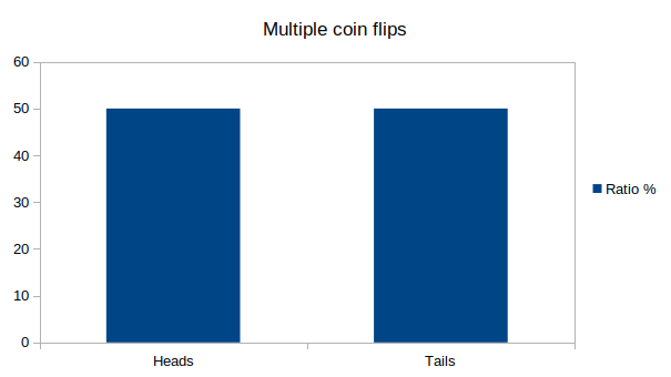
This means that on average about 50% of coin flips be heads (and tails). LLN seems deceptively simple, and it probably is, but it’s also an important observation that has many real-life applications. For example, Monte Carlo methods use this theorem. In addition, casinos can use it to guarantee long-term outcomes (and make money).

It is also important to remember that in the previous example, any individual coin flip does not depend on the previous observations. You could flip many tails, but there is no guarantee that the next flips are more likely to be heads. LLN only works with a large number of observations.

Central limit theorem

Another, perhaps more powerful, theorem is called Central Limit Theorem (CLT). This is where things get really interesting. CLT states that when we keep adding independent random variables, their normalized sum approaches normal distribution. This happens even if the random variables themselves are not normally distributed. Let’s look at the previous example again. We know that coin tosses follow an uniform distribution: getting heads or tails are equally probable. But let’s perform coin toss, say, 100 times, and look at the resulting counts for heads and tails. If this experiment is repeated enough times, interesting things happen.

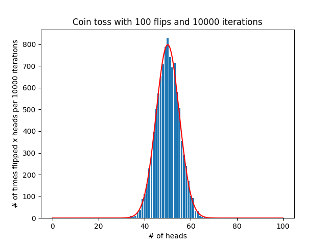
This demonstrates visually that the distribution of number of heads (or tails) indeed seems to follow normal distribution. CLT is the reason that normal distributions can be encountered almost anywhere. It is important to remember, however, that CLT makes some strong assumptions, such as the independence of random variables. In our example, the assumptions hold true and therefore the theorem works.

The cool thing about both LLN and CLT is that they are easy to demonstrate and observe by yourself. Even if you don’t believe in these theorems, it’s easy to write a piece of code that will visualize that they indeed seem to work. These are simple examples, but I think writing code that demonstrates theoretical concepts makes it easier to understand them. I’m not going to go into theoretical details about what was mentioned in this post since I’m not a statistician and there is plenty of information already out there, but I do enjoy these little coding experiments from time to time. You can find the code used to generate the example images here.