Visualizing Autoencoder Reconstruction

Autoencoders are neural networks that try to copy its input to output. The idea sounds a bit silly, but they do have applications in, e.g., denoising and dimensionality reduction.

In this post, we’ll take a look at how an autoencoder reconstructs images from the MNIST hand-written digit data.

Autoencoder

This part assumes that the reader has at least a basic understanding of what neural networks are (on an intuitive level).

As mentioned, autoencoders are neural networks that simply set the output same as the input. Then they attempt to learn the parameters of the network and minimize reconstruction error. But what is the point of that? For example, a network with a hidden layer with the same size as the input (and output) could just simply copy the inputs to the output, and have zero error. This would of course be meaningless.

But if we consider the situation where hidden layers are smaller, it’s obvious that the network needs to learn some low-dimensional representation of the data in order to reconstruct it later.

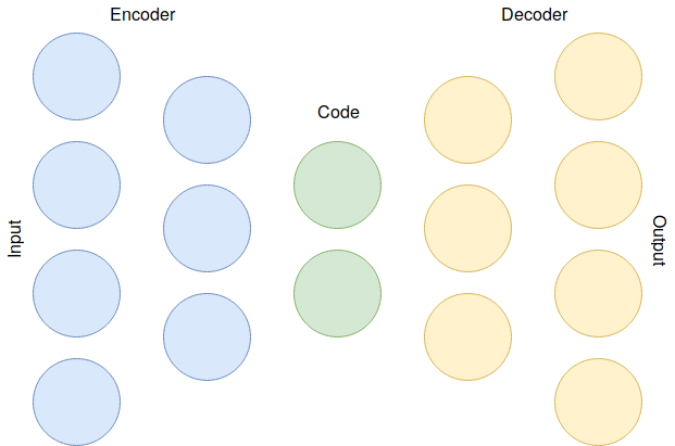
Below is a visualization of this case, including encoder and decoder parts of the network. This kind of autoencoder is called undercomplete. Encoder learns to represent the data in lower dimensions (ending up in the middle layer code). Middle layer represents the latent space. Decoder then reconstructs the data into ouput.

It is also possible to have more neurons in hidden than input layer. These types of autoencoders are overcomplete. In this case it is necessary to introduce some kind of regularization to encourage sparsity for the network to actually work.

I don’t like to go into too much detail, since a lot has been already written about autoencoders. However, it would be nice to visualize the learning process to get a better idea how it all works. Let’s do that with some TensorFlow code.

Demo with code

Full commented code can be found in this GitHub repository. Here are some simplified code snippets to demonstrate how to define an autoencoder using TensorFlow. All of the code assumes that you have TF installed and imported:

import tensorflow as tf

We can now define a model (graph) for autoencoder. This example architecture consists of 3 hidden layers with 500, 100 and 500 neurons, respectively. We can use tf.layers.dense for densely connected neural network layers. TensorFlow layers automatically take care of weight and bias initialization. Input and output tensors x and output are of the same size.

def autoencoder(x, output_size, outer_size=400, inner_size=100):
    with tf.variable_scope(name):
        encoder = tf.layers.dense(x, outer_size, name='encoder')
        code = tf.layers.dense(encoder, inner_size, name='code')
        decoder = tf.layers.dense(code, outer_size, name='decoder')
        output = tf.layers.dense(decoder, output_size, name='output')
        return output

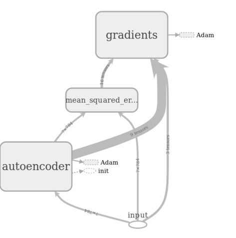
From the graph below you can see how TensorFlow constructs the network, including MSE and gradient calculation. The relevant values are fed to Adam optimizer.

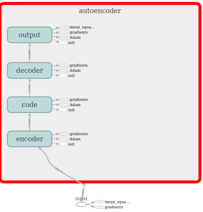
If we take a look inside the autoencoder graph, we can see that we have exactly the layers we specified in our model. From this you can also see how the MSE is only calculated from the output layer (and input layer of course, because that is the data we are trying to reconstruct).

We can load the MNIST dataset, and also select one example image for visualizing reconstruction (in this case image with index 10). With TensorFlow 1.7 and newer you have to load datasets manually, or use some other method (such as scikit learn).

#Load MNIST data (NOTE: Removed in TF 1.7)
mnist = tf.contrib.learn.datasets.load_dataset('mnist')
# Example figure to visualize
example_fig = [mnist.train.images[10]]

Next, we need to define some parameters.

# Learning rate for Adam optimizer
learning_rate = 0.001
# Images are 28*28 pixels
input_size = 28*28
# Mini-batch size
batch_size = 100
# Total number of steps
steps = 10000
# Save training loss and image every [save_every] steps
save_every = 100

Now we are actually going to do some TensorFlow coding. TF placeholder x is going to be the placeholder for our model input data. Placeholder just means that we will be replacing it with the actual data when training and running the model, it does not have any value by itself. Other often used types are constants (values which do not change) and variables (values will change, and are optimized by TensorFlow during model training, e.g., weights and biases).

We define our output op, where the autoencoder model takes our input placeholder and returns model outputs. MSE loss is used in this case, and we utilize Adam optimizer (the details of which I will get to in a later post). The train op simply uses Adam optimizer to minimize the loss that we defined, using the learning rate parameter defined previously.

# Input placeholder
x = tf.placeholder(tf.float32, [None, input_size], name='input')
# Output prediction step
output = autoencoder(x, input_size)
# Using MSE loss
loss = tf.losses.mean_squared_error(x, output)
# Train op using Adam optimizer
train_op = tf.train.AdamOptimizer(learning_rate).minimize(loss)

After initializing the TF session, we finally get to our training loop. This code uses the traditional and versatile feed dict functionality, but it’s good to note that for performance reasons other methods might be recommended, e.g., queues. Every iteration, we take a random mini-batch from MNIST data and run the training and loss operations. Every once in a while we also print the training loss and also save the image (you can do this however you want).

with tf.Session() as sess:
    init = tf.global_variables_initializer()
    sess.run(init)
    for i in range(1, steps+1):
        batch, _ = mnist.train.next_batch(batch_size)
        _, l = sess.run([train_op, loss], feed_dict={x: batch})
        if i % save_every == 0:
            print('Training loss at step {0}: {1}'.format(i, l))
            # Reconstruct example image
            result = sess.run([output], feed_dict={x: example_fig})
            # Code for saving figure here

Visualizing reconstruction

Finally we can visualize the reconstructed image. As the autoencoder gets better quite quickly, I’m only going to show the first 200 iterations. Looking at the image below, we can see how the reconstruction changes from basically noise into something much better.

In conclusion, this example does not yet explain how autoencoders can be useful. However, we see that even though an image with 784 pixels is compressed into 100 dimensions, it can still be reconstructed pretty well. It’s this latent layer that really holds the key to the usefulness of autoencoders. I will have to get back to that in a later post.