Vanishing Gradient Problem in Deep Neural Nets
In this post we are going to take a look at a problem that became an issue with the rise of deep learning: the vanishing gradient. We need to know what it is to avoid rendering our deep neural network useless. But first, let’s start with some background.
Neural network basics
I’m going to give a little of bit of background information needed to understand the problem. Some basic understanding of neural networks is useful at this point. I’m not going to go into too much detail because there are already countless resources available.
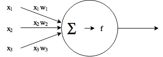
A neural network consists of neurons (or nodes). They take input data multiplied by weights and add these together. After this, the aggregated sum is input into an activation function, which determines the output of the neuron. Optimizing the weights is essentially what a neural network does when it’s learning.
A commonly used activation function is the sigmoid function:

If we plot it, it looks like this:

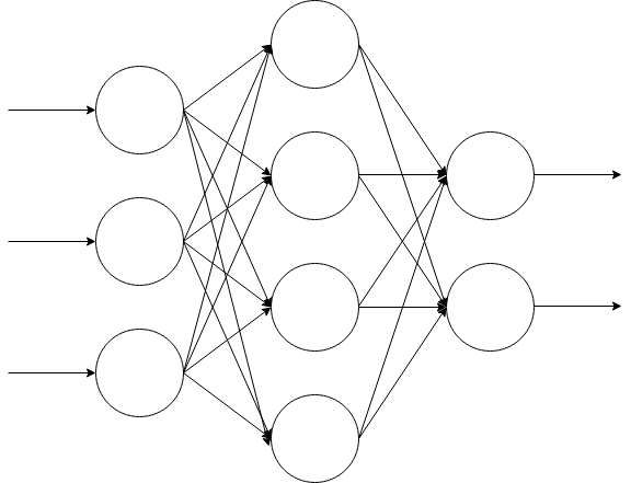
Individual neurons can be combined to form a neural network, which aims to approximate any arbitrary function. Each node in the network has its own inputs, outputs and activations. Below is an example of a simple feed-forward network. It has an input layer, hidden layer and output layer.
It is also possible to have more connections or different number of neurons in each layer. Recently it has become possible to use more layers with more computing power and the use of GPUs. This is often associated with deep learning or deep neural networks. But, with more layers a new problem arises. Let’s take a look at that next. By the way, I know that this section did not go into too much detail about neural networks. Really, there is already a lot of information on those, so I’m keeping it really short.
Backpropagation and vanishing gradient
In practice, neural network learning is done by optimizing the weights. This can be performed by using backpropagation. We check the error for each layer and adjust the weights in the appropriate direction. This error is then propagated all the way back to the first layer. To do this in practice, gradient descent algorithm is often used. We need to have a loss function. The gradient tells us which way we need to go to get smaller values for that function (if we move in the negative direction). This optimization gives us the local minimum of the loss function after some iterations.
Calculating the gradient involves the use of derivative of the activation function. We can calculate the gradient for different layers of the network using the chain rule. At this point it’s enough to know that we are basically calculating a product of derivatives. We end up multiplying n gradients for n layers in the network.
Now let’s see what the derivative of the sigmoid function looks like:
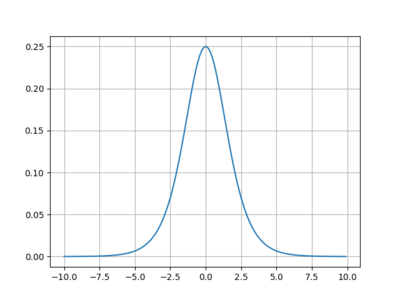
Looks like it has the maximum value of 0.25, often being much smaller than that. Now imagine a deep neural network with many layers: what is going to happen? Thus, we end up with the vanishing gradient problem. The gradient is always less than zero, so it keeps getting smaller and smaller exponentially layer by layer (or, it begins to vanish). This means that the first layers train very slowly. In practice, this means that our network becomes pretty much useless.
It’s also possible for the gradient to increase exponentially with very high gradient values. This is called exploding gradient.
What happens with a different activation function?
By this point we’ve established that the choice of activation function is very important. The sigmoid function is sort of dead in deep neural networks. What else could we use? A popular choice is rectified linear unit (ReLU). At this point it’s enough to mention that ReLU has gradient of 1 when the output is > 0, and otherwise zero. This way there we don’t have to worry about vanishing gradient anymore. The zero gradient values also create sparsity in the network, which can be a challenge but also a big advantage. The details of that are a story for another day, however.